Building the Code
This code is a reference implementation of our paper Closest Point Turbulence for Liquid Surfaces.
We have successfully built this code in Mac OSX (10.6, Snow Leopard) and Linux (Ubuntu 12.02). The default Makefile is for OSX, and the Linux Makefile is Makefile.ubuntu. We have made an effort to remove dependencies on external libraries, so aside from some commonly available libraries (zlib, libpng), you should not need to download and install anything special in order to successfully compile.
You should be able to build using the following sequence:
gunzip CPT.tar.gz
tar -xvf CPT.tar
cd CPT
make
If you are using Linux, replace the last line with make -f Makefile.ubuntu. If you are successful, the binaries iWaveHoudini and iWavePhysBAM should now be in the CPT directory.
The Houdini Example
Unfortunately, we are unable to provide a download for the low-resolution liquid files, as they are quite large (5.5 GB), even after compression.
For the Houdini example, we have instead provided the original Houdini scene file so you can regenerate the low-resolution simulation yourself. You do not need to buy Houdini;
the free Houdini Apprentice edition is fully capable of outputting the data. Once you have uncompressed the download, the scene file is located at:
CPT/data/houdini_input/paddle_example.hipnc
Open the file in Houdini, and press the Play button, the unadorned right-pointing arrowhead in the lower left hand corner. It will take a while to run, and when it is complete
there will be surf*.geo and vel_out*.geo files in the CPT/data/houdini_input directory that range from 0 to 240.
Once these files are present, execute the following from the top-most CPT directory to up-res the simulation:
The 2 argument to iWaveHoudini specifies that a 2x upres is desired. You can increase it to whatever factor you want, depending on how much time and memory you have.
Note that we have only tested with workflow using Houdini 12.5, so results may vary with different versions. In particular, the file format changed between Houdini 11 and 12, so
you need to be using at least Houdini 12.0.
The PhysBAM Example
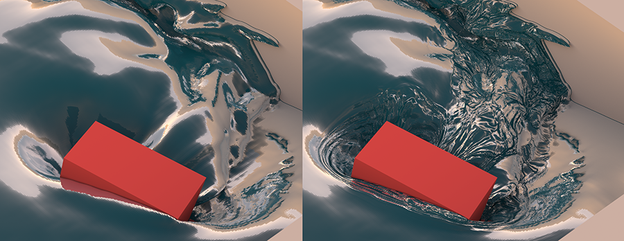
The "Pouring" example from the paper (Figure 8) is the default 3D example that is generated by the PhysBAM water project.
Download, build, and run this example (it may take some effort). Once it has completed, you should have a set of numbered directories. Copy all of these directories into:
If you are successful, there should be directory CPT/data/PhysBAM_input/1 containing all the data from the first simulation frame, CPT/data/PhysBAM_input/2 containing the data from the second frame, and so on.
Once these directories are present, execute the following from the top-most CPT directory to up-res the simulation:
As with the Houdini upres, the 2 argument specifies a 2x upes.
Rendering:
By default, the code shows an OpenGL preview window of the simulation as it is running. The underlying turbulence results are only crudely sampled for preview purposes; it does not reflect the full detail that will be present in the final renderings.
You must have PBRT 2.0 installed in order to render the final images. We have modified PBRT to support our 3D texture files, so you will need to rebuild PBRT by following the directions in CPT/render/pbrt_modifications/README.txt.
If you have successfully used iWaveHoudini and iWavePhysBAM to up-res simulation data, and you have succesfully built the modified PBRT, then you should be able to render them by going to the directory
and executing
perl render_houdini.pl 0 20
perl render_PhysBAM.pl 0 20
The 0 20 arguments to the Perl script denote that frames 0 to 20 should be rendered. If you generated more upres frames, you can increase this range.